3.3. scikit-image: 画像処理
著者: Emmanuelle Gouillart
scikit-image は画像処理専用のPythonパッケージで、NumPyの配列を画像オブジェクトとして使用します。 この章では、様々な画像処理タスクのために scikit-image を使用する方法と、NumPyやSciPyのような他の科学的なPythonモジュールとの関係について説明します。
参考
画像の切り抜きや簡単なフィルタリングのような基本的な画像操作については、NumPyとSciPyだけで多くの簡単な操作を実現することができます。 Image manipulation and processing using NumPy and SciPy を参照してください。
マスキングやラベリングといった基本的な操作が前提になるので、この章を読む前に、前の章の内容をよく理解しておく必要があることに注意してください。
3.3.1. イントロダクションとコンセプト
画像はNumPyの配列 np.ndarray です。
- 画像:
np.ndarray- ピクセル:
array values:
a[2, 3]- channels:
array dimensions
- image encoding:
dtype(np.uint8,np.uint16,np.float)- filters:
functions (
numpy,skimage,scipy)
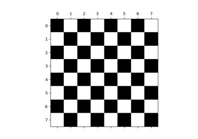
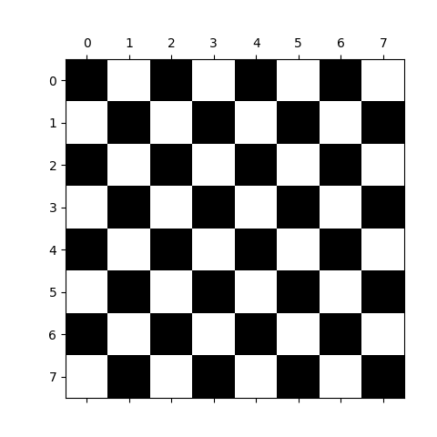
>>> import numpy as np
>>> check = np.zeros((8, 8))
>>> check[::2, 1::2] = 1
>>> check[1::2, ::2] = 1
>>> import matplotlib.pyplot as plt
>>> plt.imshow(check, cmap='gray', interpolation='nearest')
<matplotlib.image.AxesImage object at ...>
3.3.1.1. scikit-image と科学的Pythonエコシステム
scikit-image は pip と conda ベースの Python インストーラ、およびほとんどの Linux ディストリビューションでパッケージ化されています。 NumPy 配列を操作する画像処理と可視化のための他の Python パッケージには以下のものがあります:
scipy.ndimageN次元配列の場合 基本的なフィルタリング、数理形態学、領域の特性
- Mahotas
高速実装に焦点を当てています。
- Napari
Qt で作られた高速でインタラクティブな多次元画像ビューア。
いくつかの強力なC++画像処理ライブラリには、Pythonバインディングもあります:
程度の差こそあれ、これらはあまりPythonicでなくNumPyに優しくない傾向があります。
3.3.1.2. scikit-imageに含まれるもの
このライブラリには、主に画像処理アルゴリズムが含まれていますが、データの取り扱いと処理を容易にするユーティリティ関数も含まれています。 以下のサブモジュールを含みます:
color色空間の変換。
dataテスト画像とサンプルデータ。
drawNumPyの配列を操作する描画プリミティブ (線、テキストなど) 。
exposure画像強度調整、例、ヒストグラム等化など
feature特徴検出と抽出、例、テクスチャー分析コーナーなど。
filtersシャープネス、エッジ検出、ランクフィルター、閾値処理など。
graphグラフ理論的操作、例えば最短経路。
io画像やビデオの読み取り、保存、表示。
measure画像特性の測定、例えば、リージョンプロパティや輪郭など。
metrics画像に対応するメトリクス、例えば、距離メトリクス、類似度など。
morphology形態学的操作、例えば、オープニングやスケルトン化。
restoration復元アルゴリズム、例えばデコンボリューションアルゴリズム、ノイズ除去など。
segmentation画像を複数の領域に分割する。
transform幾何学変換やその他の変換、例えば回転やRadon変換など。
util汎用ユーティリティ。
3.3.2. Importing
scikit-image をインポートするには:
>>> import skimage as ski
ほとんどの機能はサブパッケージに含まれています、例えば:
>>> image = ski.data.cat()
以下ですべてのサブモジュールを一覧できます:
>>> for m in dir(ski): print(m)
__version__
color
data
draw
exposure
feature
filters
future
graph
io
measure
metrics
morphology
registration
restoration
segmentation
transform
util
ほとんどの scikit-image 関数は、NumPyの ndarrays を引数にとります
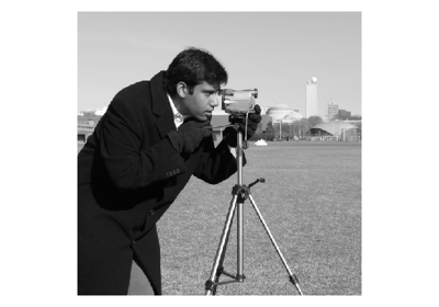
>>> camera = ski.data.camera()
>>> camera.dtype
dtype('uint8')
>>> camera.shape
(512, 512)
>>> filtered_camera = ski.filters.gaussian(camera, sigma=1)
>>> type(filtered_camera)
<class 'numpy.ndarray'>
3.3.3. データ例
手始めに、作業用のサンプル画像が必要です。 ライブラリーには、これらのうちのいくつかが同梱されています:
>>> image = ski.data.cat()
>>> image.shape
(300, 451, 3)
3.3.4. 入出力、データ型、色空間
I/O: skimage.io
画像をディスクに保存します: skimage.io.imsave()
>>> ski.io.imsave("cat.png", image)
Reading from files: skimage.io.imread()
>>> cat = ski.io.imread("cat.png")
これは、 ImageIO ライブラリーがサポートする多くのデータフォーマットで機能します。
ロードはURLでも機能します:
>>> logo = ski.io.imread('https://scikit-image.org/_static/img/logo.png')
3.3.4.1. Data types
Image ndarrays can be represented either by integers (signed or unsigned) or floats.
整数データ型でのオーバーフローに注意してください
>>> camera = ski.data.camera()
>>> camera.dtype
dtype('uint8')
>>> camera_multiply = 3 * camera
Different integer sizes are possible: 8-, 16- or 32-bytes, signed or unsigned.
警告
An important (if questionable) skimage convention: float images
are supposed to lie in [-1, 1] (in order to have comparable contrast for
all float images)
>>> camera_float = ski.util.img_as_float(camera)
>>> camera.max(), camera_float.max()
(np.uint8(255), np.float64(1.0))
Some image processing routines need to work with float arrays, and may hence output an array with a different type and the data range from the input array
>>> camera_sobel = ski.filters.sobel(camera)
>>> camera_sobel.max()
np.float64(0.644...)
Utility functions are provided in skimage to convert both the
dtype and the data range, following skimage's conventions:
util.img_as_float, util.img_as_ubyte, etc.
See the user guide for more details.
3.3.4.2. Colorspaces
Color images are of shape (N, M, 3) or (N, M, 4) (when an alpha channel encodes transparency)
>>> face = sp.datasets.face()
>>> face.shape
(768, 1024, 3)
Routines converting between different colorspaces (RGB, HSV, LAB etc.)
are available in skimage.color : color.rgb2hsv, color.lab2rgb,
etc. Check the docstring for the expected dtype (and data range) of input
images.
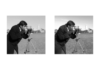
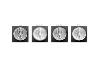
3.3.5. 画像の前処理/改良
目標: ノイズ除去、特徴(エッジ)抽出、...
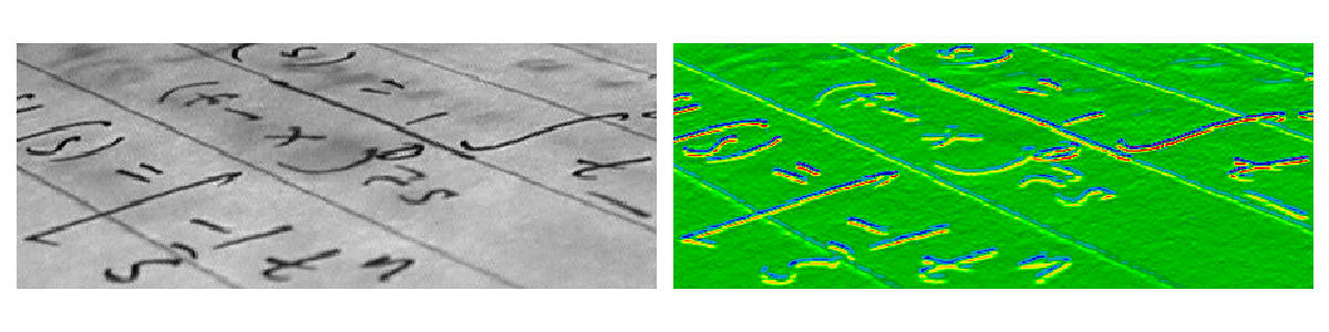
3.3.5.1. 局所フィルター
局所フィルターは、ピクセルの値を局所ピクセルの値の関数で置き換えます。この関数は線形でも非線形でもよいです。
局所: 正方形(サイズを選択)、円盤、またはより複雑な 構造要素 。
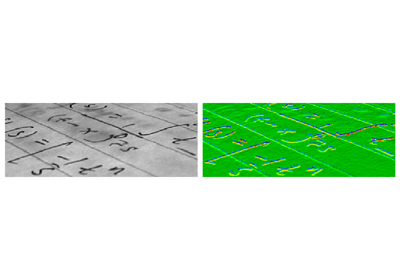
例: 水平Sobelフィルター
>>> text = ski.data.text()
>>> hsobel_text = ski.filters.sobel_h(text)
水平勾配の計算には次の線形カーネルを使用します:
1   2   1
0   0   0
-1  -2  -1
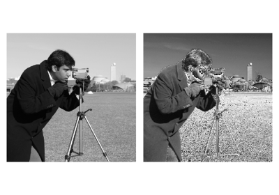
3.3.5.2. 非局所フィルター
非局所フィルターは、画像の広い領域(または画像全体)を使って、あるピクセルの値を変換します:
>>> camera = ski.data.camera()
>>> camera_equalized = ski.exposure.equalize_hist(camera)
ほぼ均一な広い領域のコントラストを高めます。
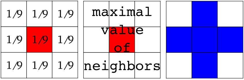
3.3.5.3. 数学的形態学
数学的形態学については wikipedia を参照してください。
単純な形状( 構造化要素 )で画像を探査し、その形状が局所的に画像にどのようにフィットするか、あるいは画像をどのように外すかによって、この画像を修正します。
Default structuring element: 4-connectivity of a pixel
>>> # Import structuring elements to make them more easily accessible
>>> from skimage.morphology import disk, diamond

>>> diamond(1)
array([[0, 1, 0],
       [1, 1, 1],
       [0, 1, 0]], dtype=uint8)
Erosion = minimum filter. Replace the value of a pixel by the minimal value covered by the structuring element.:
>>> a = np.zeros((7,7), dtype=np.uint8)
>>> a[1:6, 2:5] = 1
>>> a
array([[0, 0, 0, 0, 0, 0, 0],
       [0, 0, 1, 1, 1, 0, 0],
       [0, 0, 1, 1, 1, 0, 0],
       [0, 0, 1, 1, 1, 0, 0],
       [0, 0, 1, 1, 1, 0, 0],
       [0, 0, 1, 1, 1, 0, 0],
       [0, 0, 0, 0, 0, 0, 0]], dtype=uint8)
>>> ski.morphology.binary_erosion(a, diamond(1)).astype(np.uint8)
array([[0, 0, 0, 0, 0, 0, 0],
       [0, 0, 0, 0, 0, 0, 0],
       [0, 0, 0, 1, 0, 0, 0],
       [0, 0, 0, 1, 0, 0, 0],
       [0, 0, 0, 1, 0, 0, 0],
       [0, 0, 0, 0, 0, 0, 0],
       [0, 0, 0, 0, 0, 0, 0]], dtype=uint8)
>>> #Erosion removes objects smaller than the structure
>>> ski.morphology.binary_erosion(a, diamond(2)).astype(np.uint8)
array([[0, 0, 0, 0, 0, 0, 0],
       [0, 0, 0, 0, 0, 0, 0],
       [0, 0, 0, 0, 0, 0, 0],
       [0, 0, 0, 0, 0, 0, 0],
       [0, 0, 0, 0, 0, 0, 0],
       [0, 0, 0, 0, 0, 0, 0],
       [0, 0, 0, 0, 0, 0, 0]], dtype=uint8)
Dilation: maximum filter:
>>> a = np.zeros((5, 5))
>>> a[2, 2] = 1
>>> a
array([[0.,  0.,  0.,  0.,  0.],
       [0.,  0.,  0.,  0.,  0.],
       [0.,  0.,  1.,  0.,  0.],
       [0.,  0.,  0.,  0.,  0.],
       [0.,  0.,  0.,  0.,  0.]])
>>> ski.morphology.binary_dilation(a, diamond(1)).astype(np.uint8)
array([[0, 0, 0, 0, 0],
       [0, 0, 1, 0, 0],
       [0, 1, 1, 1, 0],
       [0, 0, 1, 0, 0],
       [0, 0, 0, 0, 0]], dtype=uint8)
Opening: erosion + dilation:
>>> a = np.zeros((5,5), dtype=int)
>>> a[1:4, 1:4] = 1; a[4, 4] = 1
>>> a
array([[0, 0, 0, 0, 0],
       [0, 1, 1, 1, 0],
       [0, 1, 1, 1, 0],
       [0, 1, 1, 1, 0],
       [0, 0, 0, 0, 1]])
>>> ski.morphology.binary_opening(a, diamond(1)).astype(np.uint8)
array([[0, 0, 0, 0, 0],
       [0, 0, 1, 0, 0],
       [0, 1, 1, 1, 0],
       [0, 0, 1, 0, 0],
       [0, 0, 0, 0, 0]], dtype=uint8)
Opening removes small objects and smoothes corners.
より高度な数学的形態学が利用できます: tophat、skeletonizationなど。
参考
基本的な数理形態学は scipy.ndimage.morphology にも実装されています。 ``scipy.ndimage``の実装は任意の次元の配列に対して動作します。
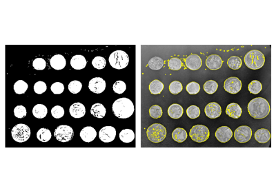
3.3.6. 画像分割
画像セグメンテーションとは、画像の異なる領域に異なるラベルを付けることであり、例えば、関心のあるオブジェクトのピクセルを抽出するために行われます。
3.3.6.1. バイナリセグメンテーション: 前景+背景
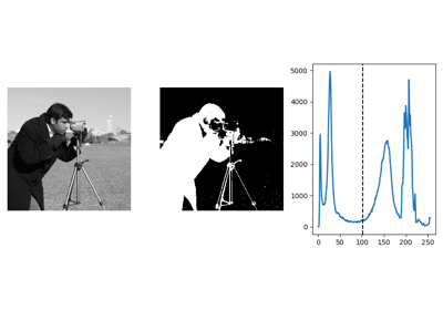
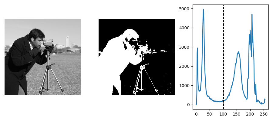
ヒストグラムに基づく方法: Otsu thresholding
Tip
Otsu method は、前景と背景を分離する閾値を見つけるための単純なヒューリスティックである。
camera = ski.data.camera()
val = ski.filters.threshold_otsu(camera)
mask = camera < val
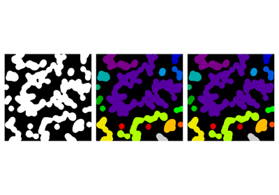
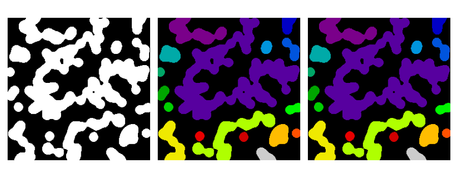
離散画像の連結成分にラベルを付ける
Tip
前景オブジェクトを分離したら、それらを互いに分離するのに使います。 そのために、それぞれに異なる整数ラベルを割り当てることができます。
合成データ:
>>> n = 20
>>> l = 256
>>> im = np.zeros((l, l))
>>> rng = np.random.default_rng()
>>> points = l * rng.random((2, n ** 2))
>>> im[(points[0]).astype(int), (points[1]).astype(int)] = 1
>>> im = ski.filters.gaussian(im, sigma=l / (4. * n))
>>> blobs = im > im.mean()
接続されているすべてのコンポーネントにラベルを貼ります:
>>> all_labels = ski.measure.label(blobs)
接続されているすべての前景コンポーネントにラベルを貼ります:
>>> blobs_labels = ski.measure.label(blobs, background=0)
参考
scipy.ndimage.find_objects() は、画像内のオブジェクトのスライスを返すのに便利です。
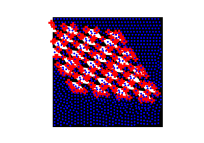
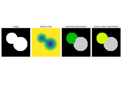
3.3.6.2. マーカーに基づく方法
リージョンのセットの中にマーカーがあれば、それを使ってリージョンを分割することができます。
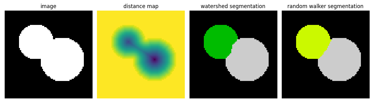
Watershed セグメンテーション
Watershed (skimage.segmentation.watershed()) は、画像の "basins " を埋める領域拡大アプローチです
>>> # Generate an initial image with two overlapping circles
>>> x, y = np.indices((80, 80))
>>> x1, y1, x2, y2 = 28, 28, 44, 52
>>> r1, r2 = 16, 20
>>> mask_circle1 = (x - x1) ** 2 + (y - y1) ** 2 < r1 ** 2
>>> mask_circle2 = (x - x2) ** 2 + (y - y2) ** 2 < r2 ** 2
>>> image = np.logical_or(mask_circle1, mask_circle2)
>>> # Now we want to separate the two objects in image
>>> # Generate the markers as local maxima of the distance
>>> # to the background
>>> import scipy as sp
>>> distance = sp.ndimage.distance_transform_edt(image)
>>> peak_idx = ski.feature.peak_local_max(
...     distance, footprint=np.ones((3, 3)), labels=image
... )
>>> peak_mask = np.zeros_like(distance, dtype=bool)
>>> peak_mask[tuple(peak_idx.T)] = True
>>> markers = ski.morphology.label(peak_mask)
>>> labels_ws = ski.segmentation.watershed(
...     -distance, markers, mask=image
... )
ランダムウォーカー セグメンテーション
ランダムウォーカーアルゴリズム (skimage.segmentation.random_walker()) はWatershedに似ていますが、より "確率的" なアプローチです。 画像内のラベルの拡散という考えに基づいています:
>>> # Transform markers image so that 0-valued pixels are to
>>> # be labelled, and -1-valued pixels represent background
>>> markers[~image] = -1
>>> labels_rw = ski.segmentation.random_walker(image, markers)
3.3.7. 領域の特性を測定する
例: 2つの分割された領域のサイズと周囲を計算します:
>>> properties = ski.measure.regionprops(labels_rw)
>>> [float(prop.area) for prop in properties]
[770.0, 1168.0]
>>> [prop.perimeter for prop in properties]
[np.float64(100.91...), np.float64(126.81...)]
参考
プロパティによっては、別のAPIで scipy.ndimage.measurements に関数が用意されています (リストが返されます) 。
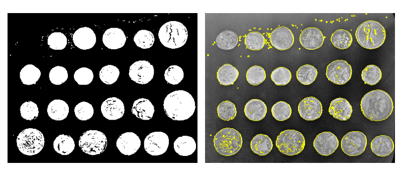
3.3.8. データの可視化とインタラクション
意味のある可視化は、与えられた処理パイプラインをテストするときに役立ちます。
いくつかの画像処理操作:
>>> coins = ski.data.coins()
>>> mask = coins > ski.filters.threshold_otsu(coins)
>>> clean_border = ski.segmentation.clear_border(mask)
バイナリ結果の可視化:
>>> plt.figure()
<Figure size ... with 0 Axes>
>>> plt.imshow(clean_border, cmap='gray')
<matplotlib.image.AxesImage object at 0x...>
輪郭の視覚化
>>> plt.figure()
<Figure size ... with 0 Axes>
>>> plt.imshow(coins, cmap='gray')
<matplotlib.image.AxesImage object at 0x...>
>>> plt.contour(clean_border, [0.5])
<matplotlib.contour.QuadContourSet ...>
専用ユーティリティ関数 skimage を使用します:
>>> coins_edges = ski.segmentation.mark_boundaries(
...     coins, clean_border.astype(int)
... )
3.3.9. コンピュータビジョンのための特徴抽出
幾何学的記述子やテクスチャ記述子は、以下の目的で画像から抽出することができます
画像の一部を分類する (例:空と建物)
異なる画像の一部を一致させます (例:物体検出)
コンピュータビジョン の他の多くのアプリケーション。
例: Harris検出器によるコーナー検出:
tform = ski.transform.AffineTransform(
    scale=(1.3, 1.1), rotation=1, shear=0.7,
    translation=(210, 50)
)
image = ski.transform.warp(
    data.checkerboard(), tform.inverse, output_shape=(350, 350)
)

coords = ski.feature.corner_peaks(
    ski.feature.corner_harris(image), min_distance=5
)
coords_subpix = ski.feature.corner_subpix(
    image, coords, window_size=13
)
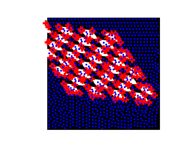
(この例はscikit-imageの plot_corner の例から引用しています)
scikit-imageの plot_matching の例で説明されているように、角のような注目点は、異なる画像内のオブジェクトをマッチングするために使用することができます。