3.4.8.14. 固有顔の例: PCAとSVMの連鎖

この例のゴールは、教師なし手法と教師あり手法をどのように連鎖させればより良い予測ができるかを示すことです。 教則的ですが長いやり方から始まり、scikit-learn のパイプラインへの慣用的なアプローチで終わります。

ここでは簡単な顔認識の例を見てみましょう。 理想的には、 sklearn.datasets.fetch_lfw_people() で利用可能な Labeled Faces in the Wild データのサブセットからなるデータセットを使うことです。 しかし、これは比較的大きなダウンロード（~200MB）なので、よりシンプルでリッチでないデータセットでチュートリアルを行うことにします。 LFWのデータセットをご自由にご覧ください。

from sklearn import datasets

faces = datasets.fetch_olivetti_faces()
faces.data.shape

downloading Olivetti faces from https://ndownloader.figshare.com/files/5976027 to /home/docs/scikit_learn_data

(400, 4096)

これらの顔を視覚化して、何を扱っているのかを見てみましょう

import matplotlib.pyplot as plt

fig = plt.figure(figsize=(8, 6))
# plot several images
for i in range(15):
    ax = fig.add_subplot(3, 5, i + 1, xticks=[], yticks=[])
    ax.imshow(faces.images[i], cmap="bone")

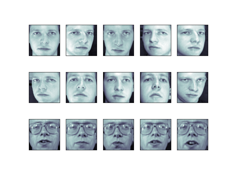
Tip

Note is that these faces have already been localized and scaled to a common size. This is an important preprocessing piece for facial recognition, and is a process that can require a large collection of training data. This can be done in scikit-learn, but the challenge is gathering a sufficient amount of training data for the algorithm to work. Fortunately, this piece is common enough that it has been done. One good resource is OpenCV, the Open Computer Vision Library.

画像のサポートベクトル分類を行います。典型的な訓練とテストの分割を画像で行います:

from sklearn.model_selection import train_test_split

X_train, X_test, y_train, y_test = train_test_split(
    faces.data, faces.target, random_state=0
)

print(X_train.shape, X_test.shape)

(300, 4096) (100, 4096)

前処理: 主成分分析

SVMにとって1850次元は多いです。 PCAを使えば、データセットの情報をほとんど維持したまま、1850の特徴を扱いやすいサイズに減らすことができます。

from sklearn import decomposition

pca = decomposition.PCA(n_components=150, whiten=True)
pca.fit(X_train)

PCA(n_components=150, whiten=True)

In a Jupyter environment, please rerun this cell to show the HTML representation or trust the notebook.
On GitHub, the HTML representation is unable to render, please try loading this page with nbviewer.org.

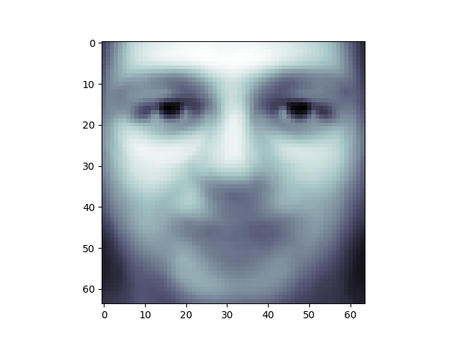
PCAの面白いところは、"平均 "顔を計算することです、 そしてそれを調べるのは興味深いことです:

plt.imshow(pca.mean_.reshape(faces.images[0].shape), cmap="bone")

<matplotlib.image.AxesImage object at 0x7b20735e11c0>

主成分は、直交する軸に沿って、この平均に関する偏差を測定します。

print(pca.components_.shape)

(150, 4096)

これらの主成分を視覚化するのも興味深いです:

fig = plt.figure(figsize=(16, 6))
for i in range(30):
    ax = fig.add_subplot(3, 10, i + 1, xticks=[], yticks=[])
    ax.imshow(pca.components_[i].reshape(faces.images[0].shape), cmap="bone")

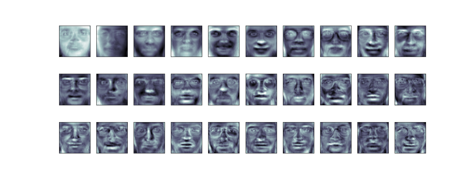
成分（"固有顔"）は、左上から右下に向かって重要度が高い順に並べられています。 最初のいくつかのコンポーネントは、主に照明条件を管理しているようです; 残りのコンポーネントは、特定の識別機能を引き出します: 鼻、目、眉毛などです。

この射影が計算されたので、元の訓練データとテストデータをPCA基底に射影することができます:

X_train_pca = pca.transform(X_train)
X_test_pca = pca.transform(X_test)
print(X_train_pca.shape)

(300, 150)

print(X_test_pca.shape)

(100, 150)

これらの投影された成分は、組み合わせが元の顔に近づくような成分画像の線形結合の因子に対応します。

学びを実践する: サポートベクターマシン

では、この縮小されたデータセットに対してサポートベクトルマシン分類を実行しましょう:

from sklearn import svm

clf = svm.SVC(C=5.0, gamma=0.001)
clf.fit(X_train_pca, y_train)

SVC(C=5.0, gamma=0.001)

In a Jupyter environment, please rerun this cell to show the HTML representation or trust the notebook.
On GitHub, the HTML representation is unable to render, please try loading this page with nbviewer.org.

最後に、この分類がどの程度うまくいったかを評価することができます。まず、トレーニングセットから学習したラベルを使って、いくつかのテストケースをプロットしてみましょう:

import numpy as np

fig = plt.figure(figsize=(8, 6))
for i in range(15):
    ax = fig.add_subplot(3, 5, i + 1, xticks=[], yticks=[])
    ax.imshow(X_test[i].reshape(faces.images[0].shape), cmap="bone")
    y_pred = clf.predict(X_test_pca[i, np.newaxis])[0]
    color = "black" if y_pred == y_test[i] else "red"
    ax.set_title(y_pred, fontsize="small", color=color)

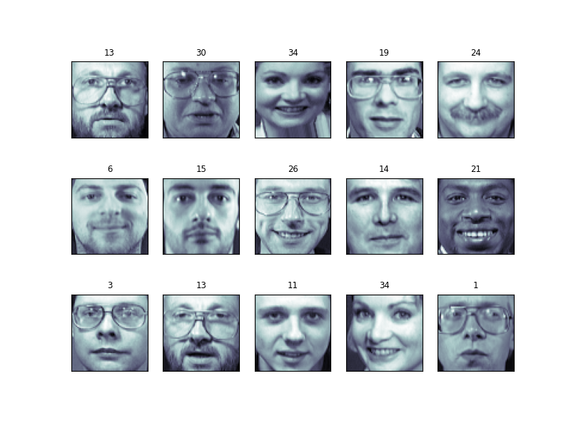
この分類器は、その学習モデルが単純であることを考えると、驚くほど多くの画像で正しいです！ ピクセルレベルのデータから導き出された150の特徴に線形分類器を用いることで、このアルゴリズムは画像内の多数の人物を正しく識別しました。

この効果も、 sklearn.metrics が提供するいくつかの指標のいずれかを使って定量化することができる。 まず、分類レポートを作成し、精度、リコール、その他分類の "良さ "を示す尺度を表示します:

from sklearn import metrics

y_pred = clf.predict(X_test_pca)
print(metrics.classification_report(y_test, y_pred))

              precision    recall  f1-score   support

           0       1.00      0.50      0.67         6
           1       1.00      1.00      1.00         4
           2       0.50      1.00      0.67         2
           3       1.00      1.00      1.00         1
           4       0.33      1.00      0.50         1
           5       1.00      1.00      1.00         5
           6       1.00      1.00      1.00         4
           7       1.00      0.67      0.80         3
           9       1.00      1.00      1.00         1
          10       1.00      1.00      1.00         4
          11       1.00      1.00      1.00         1
          12       0.67      1.00      0.80         2
          13       1.00      1.00      1.00         3
          14       1.00      1.00      1.00         5
          15       1.00      1.00      1.00         3
          17       1.00      1.00      1.00         6
          19       1.00      1.00      1.00         4
          20       1.00      1.00      1.00         1
          21       1.00      1.00      1.00         1
          22       1.00      1.00      1.00         2
          23       1.00      1.00      1.00         1
          24       1.00      1.00      1.00         2
          25       1.00      0.50      0.67         2
          26       1.00      0.75      0.86         4
          27       1.00      1.00      1.00         1
          28       0.67      1.00      0.80         2
          29       1.00      1.00      1.00         3
          30       1.00      1.00      1.00         4
          31       1.00      1.00      1.00         3
          32       1.00      1.00      1.00         3
          33       1.00      1.00      1.00         2
          34       1.00      1.00      1.00         3
          35       1.00      1.00      1.00         1
          36       1.00      1.00      1.00         3
          37       1.00      1.00      1.00         3
          38       1.00      1.00      1.00         1
          39       1.00      1.00      1.00         3

    accuracy                           0.94       100
   macro avg       0.95      0.96      0.94       100
weighted avg       0.97      0.94      0.94       100

もう一つの興味深い指標は、 混同行列 です、 これは、2つのアイテムが混在する頻度を示します。 完全な分類器の混同行列は、対角線上に0でない項目のみを持ち、非対角線上に0を持ちます:

print(metrics.confusion_matrix(y_test, y_pred))

[[3 0 0 ... 0 0 0]
 [0 4 0 ... 0 0 0]
 [0 0 2 ... 0 0 0]
 ...
 [0 0 0 ... 3 0 0]
 [0 0 0 ... 0 1 0]
 [0 0 0 ... 0 0 3]]

パイプライン

上記では、サポートベクターマシン分類器を適用する前の前処理としてPCAを使用しました。 1つの推定器の出力を2番目の推定器の入力に直接差し込むのは、よく使われるパターンです; そのため scikit-learn はこの処理を自動化する Pipeline オブジェクトを提供しています。 上記の問題は、次のようにパイプラインとして再表現できます:

from sklearn.pipeline import Pipeline

clf = Pipeline(
    [
        ("pca", decomposition.PCA(n_components=150, whiten=True)),
        ("svm", svm.LinearSVC(C=1.0)),
    ]
)

clf.fit(X_train, y_train)

y_pred = clf.predict(X_test)
print(metrics.confusion_matrix(y_pred, y_test))
plt.show()

[[4 0 0 ... 0 0 0]
 [0 4 0 ... 0 0 0]
 [0 0 1 ... 0 0 0]
 ...
 [1 0 0 ... 3 0 0]
 [0 0 0 ... 0 1 0]
 [0 0 0 ... 0 0 3]]

顔認識に関するメモ

ここでは、顔認識の前処理としてPCA "固有顔" を使用しました。 これを選んだ理由は、PCAが広く適用可能な技法であり、さまざまな種類のデータに有効だからです。 特に顔認識分野の研究、しかし、他のもっと特殊な特徴抽出法の方がはるかに効果的であることが示されています。