3.4.8.11. カリフォルニア州の住宅データに対する単純回帰分析

ここでは，カリフォルニア州の住宅データについて，単純回帰分析を行い，2種類の回帰因子を探索します。

from sklearn.datasets import fetch_california_housing

data = fetch_california_housing(as_frame=True)

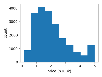
予測する数量のヒストグラムを表示: 価格

import matplotlib.pyplot as plt

plt.figure(figsize=(4, 3))
plt.hist(data.target)
plt.xlabel("price ($100k)")
plt.ylabel("count")
plt.tight_layout()

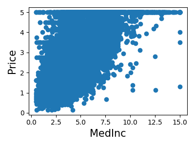
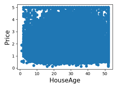
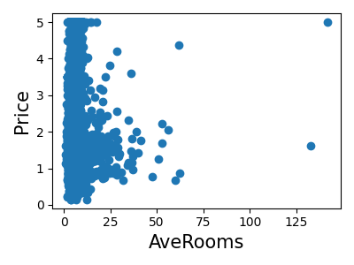
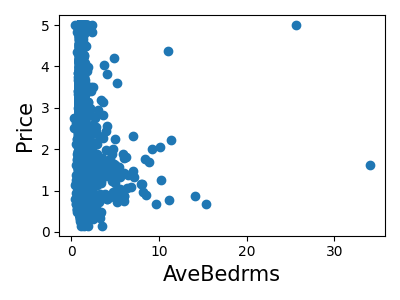
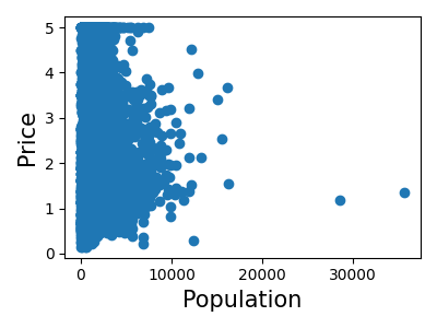
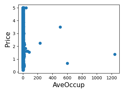
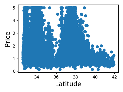
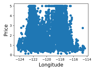
各特徴の結合ヒストグラムを表示します

for index, feature_name in enumerate(data.feature_names):
    plt.figure(figsize=(4, 3))
    plt.scatter(data.data[feature_name], data.target)
    plt.ylabel("Price", size=15)
    plt.xlabel(feature_name, size=15)
    plt.tight_layout()

• 
• 
• 
• 
• 
• 
• 
• 

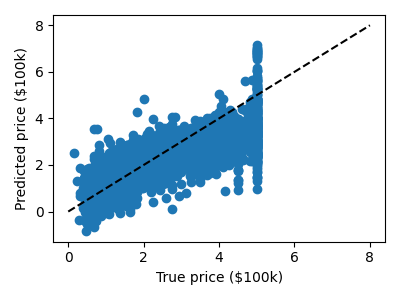
単純な予測をします

from sklearn.model_selection import train_test_split

X_train, X_test, y_train, y_test = train_test_split(data.data, data.target)

from sklearn.linear_model import LinearRegression

clf = LinearRegression()
clf.fit(X_train, y_train)
predicted = clf.predict(X_test)
expected = y_test

plt.figure(figsize=(4, 3))
plt.scatter(expected, predicted)
plt.plot([0, 8], [0, 8], "--k")
plt.axis("tight")
plt.xlabel("True price ($100k)")
plt.ylabel("Predicted price ($100k)")
plt.tight_layout()

勾配ブースティング木による予測

from sklearn.ensemble import GradientBoostingRegressor

clf = GradientBoostingRegressor()
clf.fit(X_train, y_train)

predicted = clf.predict(X_test)
expected = y_test

plt.figure(figsize=(4, 3))
plt.scatter(expected, predicted)
plt.plot([0, 5], [0, 5], "--k")
plt.axis("tight")
plt.xlabel("True price ($100k)")
plt.ylabel("Predicted price ($100k)")
plt.tight_layout()

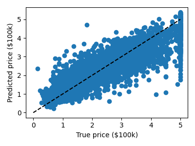
エラー率を表示します

import numpy as np

print(f"RMS: {np.sqrt(np.mean((predicted - expected) ** 2))!r} ")

plt.show()

RMS: np.float64(0.5314909993118918)